AI Fundamentals

Intro to Machine Learning

Definitions and Distinctions

In CS, the terms “Artificial Intelligence” and “Machine Learning” are often used interchangeably, leading to confusion. While closely related, they represent distinct concepts with specific applications and theoretical underpinnings.

Artificial Intelligence

AI is a broad field focused on developing intelligent systems capable of performing tasks that typically require human intelligence. These tasks include understanding natural language, recognizing objects, making decisions, solving problems, and learning from experience. AI systems exhibit cognitive abilities like reasoning, perception, and problem-solving across various domains. Some key areas of AI include:

• Natural Language Processing (NLP): Enabling computers to understand, interpret, and generate human language.
• Computer Vision: Allowing computers to “see” and interpret images and videos.
• Robotics: Developing robots that can perform tasks autonomously or with human guidance.
• Expert Systems: Creating systems that mimic the decision-making abilities of human experts.

One of the primary goals of AI is to augment human capabilities, not just replace human efforts. AI systems are designed to enhance human decision-making and productivity, providing support in complex data analysis, prediction, and mechanical tasks.

Machine Learning

ML is a subfield of AI that focuses on enabling systems to learn from data and improve their performance on specific tasks without explicit programming. ML algorithms use statistical techniques to identify patterns, trends, and anomalies within datasets, allowing the system to make predictions, decisions, or classifications based on new input data.

ML can be categorized into three main types:

• Supervised Learning: The algorithm learnes from labeled data, where each data point is associated with a known outcome or label.
  • Image classification
  • Spam detection
  • Fraud prevention
• Unsupervised Learning: The algorithm learns from unlabeled data without providing an outcome or label.
  • Customer segmentation
  • Anomaly detection
  • Dimensionality reduction
• Reinforcement Learning: The algorithm learns through trial and error by interacting with an environment and receiving feedback as rewards or penalties.
  • Game playing
  • Robotics
  • Autonomous driving

ML is a rapidly evolving field with new algorithms, techniques, and applications emerging. It is a crucial enabler of AI, providing the learning and adaption capabilities that underpin many intelligent systems.

Deep Learning

DL is a subfield of ML that uses neural networks with multiple layers to learn and extract features from complex data. These deep neural networks can automatically identify intricate patterns and representations within large datasets, making them particularly powerful for tasks involving unstructured or high-dimensional data, such as images, audios, and text.

Key characteristics include:

• Hierarchical Feature Learning: DL models can learn hierarchical data representations, where each layer captures increasingly abstract features. For example, lower layers might detect edges and textures in image recognition, while higher layers identify more complex structures like shapes and objects.
• End-to-End Learning: DL models can be trained end-to-end, meaning they can directly map raw input data to desired outputs without manual feature engineering.
• Scalability: DL models can scale well with large datasets and computational resources, making them suitable for big data applications.

Common types of neural networks used in DL include:

• Convolutional Neural Networks (CNNs): Specialized for image and video data, CNNs use convolutional layers to detect local patterns and spatial hierarchies.
• Recurrent Neural Networks (RNNs): Designed for sequential data like text and speech, RNNs have loops that allow information to persist across time steps.
• Transformers: A recent advancement in DL, transformers are particularly effective for natural language processing tasks. They leverage self-attention mechanisms to handle long-range dependencies.

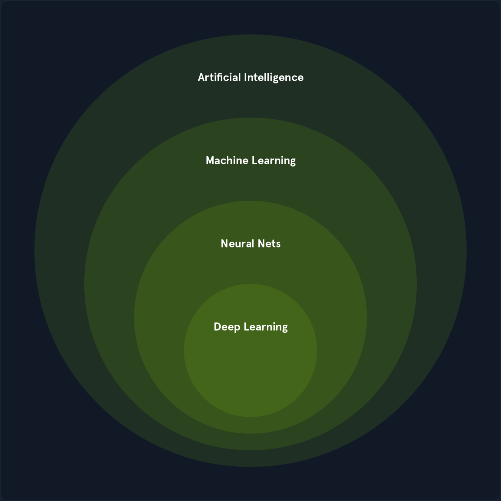
The Relationship between AI, ML, and DL

ML and DL are subfields of AI that enable systems to learn from data and make intelligent decisions. They are crucial enablers of AI, providing the learning and adaption capabilities that underpin many intelligent systems.

ML algorithms, including DL algorithms, allow machines to learn from data, recognize patterns, and make decisions. The various types of ML, such as supervised, unsupervised, and reinforcement learning, each contribute to achieving AI’s broader goals. For instance:

• In computer vision, supervised learning algorithms and deep convolutional neural networks enable machines to “see” and interpret images accurately.
• In natural language processing, traditional ML algorithms and advanced DL models like transformers allow for understanding and generating human language, enabling applications like chatbots and translation services.

DL has significantly enhanced the capabilities of ML by providing powerful tools for feature extraction and representation learning, particularly in domains with complex, unstructured data.

The synergy between ML, DL, and AI is evident in their collaborative efforts to solve complex problems. For example:

• In autonomous driving, a combination of ML and DL techniques processes sensor data, recognizes objects, and makes real-time decisions, enabling vehicles to navigate safely.
• In robotics, reinforcement learning algorithms, often enhanced with DL, train robots to perform complex tasks in dynamic environments.

ML and DL fuel AI’s ability to learn, adapt, and evolve, driving progress across various domains and enhancing human cababilities. The synergy between these fields is essential for advancing the frontiers of AI and unlocking new levels of innovation and productivity.

Mathematics Refresher

Basic Arithmetic Operations

Multiplication

The multiplication operator denotes the product of two numbers or expressions.

3 * 4 = 12

Division

The division operator denotes dividing one number or expression by another.

10 / 2 = 5

Addition

The addition operator represents the sum of two or more numbers or expressions.

5 + 3 = 8

Subtraction

The subtraction operator represents the difference between two numbers or expressions.

9 - 4 = 5

Algebraic Notations

Subscript Notation

The subscript notation represents a variable indexed by t, often indicating a specific time step or state in a sequence.

x_t = q(x_t | x_{t-2})

This notation is commonly used in sequences and time series data, where each x_t represents the value of x at time t.

Superscript Notation

Superscript notation is used to denote exponents or powers.

x^2 = x * x

This notation is used in polynomial expressions and exponential functions.

Norm

The norm measures the size or length of a vector. The most common norm is the Euclidean norm, which is calculated as follows:

||v|| = sqrt{v_1^2 + v_2^2 + ... + v_n^2}

Other norms include the L1 norm and the L∞ norm.

||v||_1 = |v_1| + |v_2| + ... + |v_n|
||v||_∞ = max(|v_1|, |v_2|, ..., |v_n|)

Norms are used in various applications, such as measuring the distance between vectors, regularizing models to prevent overfitting, and normalizing data.

Summation Symbol

The summation symbol indicates the sum of a sequence of terms.

Σ_{i=1}^{n} a_i

This represents the sum of the terms a_1, a_2, ..., a_n. Summation is used in many mathematical formulas, including calculating means, variances, and series.

Logarithms and Exponentials

Logarithms Base 2

The logarithm base 2 is the logarithm of x with base 2, often used in information theory to measure entropy.

log2(8) = 3

Logarithms are used in information theory, cryptography, and algorithms for their properties in reducing large numbers and handling exponential growth.

Natural Logarithm

The natural logarithm is the logarithm of x with base e.

ln(e^2) = 2

Due to its smooth and continous nature, the natural logarithm is widely used in calculus, differential equations, and probability theory.

Exponential Function

The exponential function represents Euler’s number e raised to the power of x.

e^{2} ≈ 7.389

The exponential function is used to model growth and decay processes, probability distributions, and various mathematical and physical models.

Exponential Function (Base 2)

The exponential function (base 2) represents 2 raised to the power of x, often used in binary systems and information metrics.

2^3 = 8

This function is used in CS, particularly in binary representations and information theory.

Matrix and Vector Operations

Matrix-Vector Multiplication

Matrix-vector multiplication denotes the product of a matrix A and a vector v.

A * v = [ [1, 2], [3, 4] ] * [5, 6] = [17, 39]

This operation is fundamental in linear algebra and is used in various applications, including transforming vectors, solving systems of linear equations, and in neural networks.

Matrix-Matrix Multiplication

Matrix-matrix multiplication denotes the product of two matrices A and B.

A * B = [ [1, 2], [3, 4] ] * [ [5, 6], [7, 8] ] = [ [19, 22], [43, 50] ]

This operation is used in linear transformations, solving systems of linear equations, and deep learning for operations between layers.

Transpose

The transpose of a matrix A is denoted by A^T and swaps the rows and columns of A.

A = [ [1, 2], [3, 4] ]
A^T = [ [1, 3], [2, 4] ]

The transpose is used in various matrix operations, such as calculating the dot product and preparing data for certain algorithms.

Inverse

The inverse of a matrix A is denoted by A^{-1} and is the matrix that, when multiplied by A, results in the identity matrix.

A = [ [1, 2], [3, 4] ]
A^{-1} = [ [-2, 1], [1.5, -0.5] ]

The inverse is used to solve systems of linear equations, inverting transformations, and various optimization problems.

Determinant

The determinant of a square matrix A is a scalar value that can be computed and is used in various matrix operations.

A = [ [1, 2], [3, 4] ]
det(A) = 1 * 4 - 2 * 3 = -2

The determinant determines whether a matrix is invertible (non-zero determinant) in calculating volumes, areas, and geometric transformations.

Trace

The trace of a square matrix A is the sum of the elements on the main diagonal.

A = [ [1, 2], [3, 4] ]
tr(A) = 1 + 4 = 5

The trace is used in various matrix properties and in calculcating eigenvalues.

Set Theory

Cardinality

The cardinality represents the number of elements in a set S.

S = {1, 2, 3, 4, 5}
|S| = 5

Cardinality is used in counting elements, probability calculations, and various combinatorial problems.

Union

The union of two sets A and B is the set of all elements in either A or B or both.

A = {1, 2, 3}, B = {3, 4, 5}
A ∪ B = {1, 2, 3, 4, 5}

The union is used in combining sets, data merging, and in various set operations.

Intersection

The intersection of two sets A and B is the set of all elements in both A and B.

A = {1, 2, 3}, B = {3, 4, 5}
A ∩ B = {3}

The intersection finds common elements, data filerting, and various set operations.

Complement

The complement of a set A is the set of all elements not in A.

U = {1, 2, 3, 4, 5}, A = {1, 2, 3}
A^c = {4, 5}

The complement is used in set operations, probability calculations, and various logical operations.

Comparison Operators

Greater Than or Equal to

The greater than or equal to operator indicates that the value on the left is either greater than or equal to the value on the riht side.

a >= b

Less Than or Equal to

The less than or equal to operator indicates that the value on the left is either less than or equal to the value on the right.

a <= b

Equality

The equality operator checks if two values are equal.

a == b

Inequality

The inequality operator checks if two values are not equal.

a != b

Eigenvalues and Scalars

Lambda

The lambda symbol often represents an eigenvalue in linear algebra or a scalar parameter in equations.

A * v = λ * v, where λ = 3

Eigenvalues are used to understand the behavior of linear transformations, principal component analysis, and various optimization problems.

Eigenvector

An eigenvector is a non-zero vector that, when multiplied by a matrix, results in a scalar multiple of itself. The scalar is the eigenvalue.

A * v = λ * v

Eigenvectors are used to understand the directions of maximum variance in data, dimensionality reduction techniques like PCA, and various machine learning algorithms.

Functions and Operators

Maximum Function

The maximum function returns the largest value from a set of values.

max(4, 7, 2) = 7

The maximum function is used in optimization, finding the best solution, and in various decision-making processes.

Minimum Function

The minimum function returns the smallest value from a set of values.

min(4, 7, 2) = 2

The minimum function is used in optimization, finding the best solution, and in various decision-making processes.

Reciprocal

The reciprocal represents one divided by an expression, effectively inverting the value.

1 / x where x = 5 results in 0.2

The reciprocal is used in various mathematical operations, such as calculating rates and proportions.

Ellipsis

The ellipsis indicates the continuation of a pattern or sequence, often used to denote an indefinte or ongoing process.

a_1 + a_2 + ... + a_n

The ellipsis is used in mathematical notation to represent sequences and series.

Functions and Probability

Function Notation

Function notation represents a function f applied to an input x.

f(x) = x^2 + 2x + 1

Function notation is used in defining mathematical relationships, modelling real-world phenomena, and in various algorithms.

Conditional Probability Distribution

The conditional probability distribution denotes the probability distributions of x given y.

P(Output | Input)

Conditional probabilities are used in Bayesian inference, decision-making under uncertainty, and various probabilistic models.

Expectation Operator

The expectation operator represents a random variable’s expected value or average over its probability distribution.

E[X] = sum x_i P(x_i)

This expectation is used in calculating the mean, decision-making under uncertainty, and various statistical models.

Variance

Variance measures the spread of a random variable X around its mean.

Var(X) = E[(X - E[X])^2]

The variance is used to understand the dispersion of data, assess risk, and use various statistical models.

Standard Deviation

Standard deviation is the square root of the variance and provides a measure of the dispersion of a random variable.

σ(X) = sqrt(Var(X))

Standard deviation is used to understand the spread of data, assess risk, and use various statistical models.

Covariance

Covariance measues how two random variables X and Y vary.

Cov(X, Y) = E[(X - E[X])(Y - E[Y])]

Covariance is used to understand the relationship between two variables, portfolio optimization, and various statistical models.

Correlation

The correlation is a normalized measure, ranging from -1 to 1. It indicates the strength and direction of the linear relationship between two random variables.

ρ(X, Y) = Cov(X, Y) / (σ(X) * σ(Y))

Correlation is used to understand the linear relationship between two variables in data analysis and in various statistical models.

Supervised Learning Algorithms

Supervised Learning Algorithms

… algorithms form the cornerstone of many ML applications, enabling systems to learn from labeled data and make accurate predictions. Each data point is associated with a known outcome or label in supervised learning. Think of it as having a set of examples with the correct answers already provided.

How Supervised Learning Works

Imagine you’re teaching a child to identify different fruits. You show them an apple and say, “This is an apple”. You then show them an orange and say, “This is an orange”. By repeatedly presenting examples with labels, the child learns to distinguish between the fruits based on their characteristics, such as color, shape, and size.

Supervised learning algorithms work similarly. They are fed with a large dataset of labeled examples, and they use this data to train a model that can predict the labels for new, unseen examples. The training process involves adjusting the model’s parameters to minimize the difference between its predictions and the actual labels.

Supervised learning problems can be broadly categorized into two main types:

1. Classification: In classification problems, the goal is to predict a categorical label. For example, classifying emails as spam or not or identifying images of cats, dogs, or birds.
2. Regression: In regression problems, the goal is to predict a continuous value. For example, one could predict the price of a house based on its size, location, and other features or forecast the stock market.

Core Concepts in Supervised Learning

Understanding supervised learning’s core concepts is essential for effectively grasping it. These concepts for the building blocks for comprehending how algorithms learn from labeled data to make accurate predictions.

Training Data

… is the foundation of supervised learning. It is the labeled dataset used to train the ML model. This dataset consists of input features and their corresponding output lables. The quality and quantity of training data significantly impact the model’s accuracy and ability to generalize to new, unseen data.

Think of training data as a set of example problems with their correct solutions. The algorithm learns from these examples to develop a model that can solve similar problems in the future.

Features

… are the measurable properties or characteristics of the data that serve as input to the model. They are the variables that the algorithm uses to learn and make predictions. Selecting relevant features is crucial for building an effective model.

For example, when predicting house prices, features might include:

• Size
• Number of bedrooms
• Location
• Age of the house

Labels

… are the known outcomes or target variables associated with each data point in the training set. They represent the “correct answers” that the model aims to predict.

In the house price prediction, the label would be the actual price of the house.

Model

A model is a mathematical representation of the relationship between the features and the labels. It is learned from the training data and used to predict new, unseen data. The model can be considered a function that takes the features as input and outputs a prediction for the label.

Training

… is the process of feeding the training data to the algorithm and adjusting the model’s parameters to minimize prediction errors. The algorithm learn from the training data by iteratively adjusting its internal parameters to imporve its prediction accuracy.

Prediction

Once the model is trained, it can be used to predict new, unseen data. This involves providing the model with features of the new data point, and the model will output a prediction for the label. Prediction is a specific application of inference, focusing on generating actionable outputs such as classifying an email as spam or forecasting stock prices.

Inference

… is a broader concept that encompasses prediciton but also inlcudes understanding the underlying structure and patterns in the data. It involves using a trained model to derive insights, estimate parameters, and understand relationships between variables.

For example, inference might involve determining which features are most important in a decision tree, estimating the coefficients in a linear regression model, or analyzing how different inputs impact the model’s prediction. While prediction emphasizes actionable outputs, inference often focuses on explaining and interpreting the results.

Evaluation

… is a critical step in supervised learning. It involves assessing the model’s performance to determine its accuracy and generalization ability to new data. Common evaluation metrics include:

• Accuracy: The proportion of correct predictions made by the model.
• Precision: The proportion of true positive predictions among all positive predictions.
• Recall: The proportion of true positive predictions among all actual positive instances.
• F1-Score: A harmonic mean of precision and recall, providing a balanced measure of the model’s performance.

Generalization

… refers to the model’s ability to accurately predict outcomes for new, unseen data not used during training. A model that generalizes well can effectively apply its learned knowledge to real-world scenarios.

Overfitting

… occurs when a model learns the training data too well, including noise and outliers. This can lead to poor generalization of new data, as the model has memorized the training set instead of learning the underlying patterns.

Underfitting

… occurs when a model is too simple to capture the underlying patterns in the data. This results in poor performance on both the training data and new, unseen data.

Cross-Validation

… is a technique used to assess how well a model will generalize to an independent dataset. It involves splitting the data into multiple subsets (folds) and training the model on different combinations of these folds while validating it on the remaining fold. This helps reduce overfitting and provides a more reliable estimate of the model’s performance.

Regularization

… is a technique used to prevent overfitting by adding a penalty to the loss function. This penalty discourages the model from learning overly complex patterns that might not generalize well. Common regularization techniques include:

• L1 Regularization: Adds a penalty equal to the absolute value of the magnitude of coefficients.
• L2 Regularization: Adds a penalty equal to the square of the magnitude of coefficients.

Linear Regression

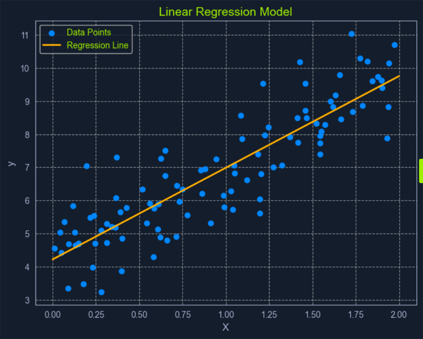
Linear Regression is a fundamental supervised learning algorithm that predicts a continuous target variable by establishing a linear relationship between the target and one or more predictor variables. The algorithm models this relationship using a linear equation, where changes in the predictor variables result in proportional changes in the target variable. The goal is to find the best-fitting line that minimizes the sum of the squared differences between the predicted values and the actual values.

Imagine you’re trying to predict a house’s price based on size. Linear regression would attempt to find a straight line that best captures the relationship between these two variables. As the size of the house increases, the price generally tends to increase. Linear regression quantifies this relationship, allowing you to predict the price of a house given its size.

What is Regression?

Regression analysis is a type of supervised learning where the goal is to predict a continuous target variable. This target variable can take on any value within a given range. Think of it as estimating a number instead of classifying something into categories.

Examples of regression problems include:

• Predicting the price of a house based on its size, location, and age.
• Forecasting the daily temperature based on historical weather data.
• Estimating the number of website visitors based on marketing spend and time of year.

In all these cases, the output you’re trying to predict is a continuous value. This is what distinguishes regression from classification, where the output is a categorical label.

Linear regression is simply one specific type of regression analysis where you assume a linear relationship between the predictor variabels and the target variables. This means you try to model the relationship using a straight line.

Simple Linear Regression

In its simplest form, simple linear regression involves one predictor variable and one target variable. A linear equation represents the relationship between them:

y = mx + c

Where:

• y is the predicted target variable
• x is the predictor variable
• m is the slope of the line (representing the relationship between x and y)
• c is the y-intercept (the value of y when is 0)

The algorithm aims to find the optimal values for m and c that minimizes the error between the predicted y values and the actual y values in the training data. This is typically done using Ordinary Least Squares (OLS), which aims to minimize the sum of squared errors.

Multiple Linear Regression

When multiple predictor variables are invovled, it’s called multiple linear regression. The equation becomes:

y = b0 + b1x1 + b2x2 + ... + bnxn

Where:

• y is the predicted target variable
• x1, x2, …, xn are the predictor variables
• b0 is the y-intercept
• b1, b2, …, bn are the coefficients representing the relationship between each predictor variable and the target variable

Ordinary Least Squares (OLS) is a common method for estimating the optimal value for the coefficients in linear regression. It aims to minimize the sum of the squared differences between the actual values and the values predicted by the model.

Think of it as finding the line that minimizes the total area of the squares formed between the data points and the line. This “line of best fit” represents the relationship that best describes the data.

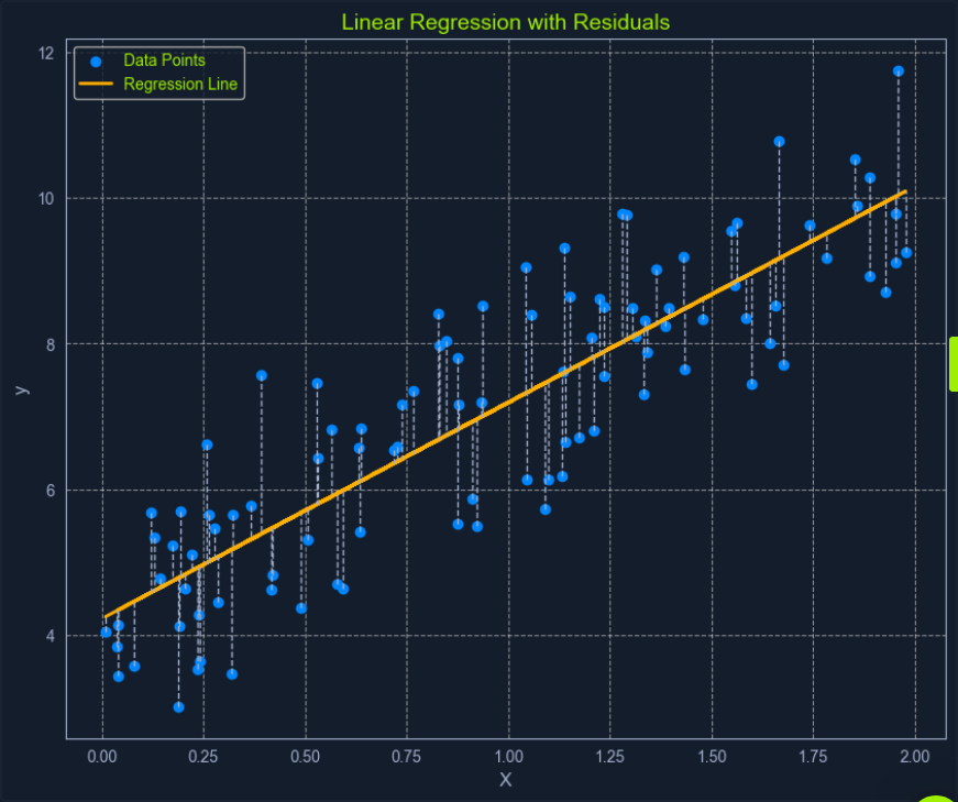
Here’s a breakdown of the OLS process:

1. Calculate Residuals: For each data point, the residual is the difference between the actual y value and the y value predicted by the model.
2. Square the Residuals: Each residual is squared to ensure that all values are positive and to give more weight to larger errors.
3. Sum the Squared Residuals: All the squared residuals are summed to get a single value representing the model’s overall error. This sum is called the Residual Sum of Squares (RSS).
4. Minimize the Sum of Squared Residuals: The algorithm adjusts the coefficients to find the values that result in the smallest possible RSS.

This process can be visualized as finding the line that minimizes the total area of the squares formed between the data points and the line.

Assumption of Linear Regression

Linear regression relies on several key assumptions about the data.

• Linearity: A linear relationship exists between the predictor and target variables.
• Independence: The observations in the dataset are independent of each other.
• Homoscedasticity: The variance of the errors is constant across all levels of the predictor variables. This means the spread of the residuals should be roughly the same across the range of predicted values.
• Normality: The errors are normally distributed. This assumption is important for making valid inferences about the model’s coefficients.

Assessing these assumptions before applying linear regression ensures the model’s validity and reliability. If these assumptions are violated, the model’s predictions may be inaccurate or misleading.